
AI AI-05.05
The transformer block
Attention plus a feed-forward network, wrapped in residual connections and layer norm: the residual stream, pre-norm, stacking, and parameter-count math.
The big idea
Attention lets tokens exchange information, but it only computes weighted averages. A model also needs to think about what it gathered: combine features, apply facts it has memorised, transform "subject of a verb" plus "plural" into a prediction. A transformer blockThe repeating unit of a transformer: multi-head attention followed by a position-wise feed-forward network, each wrapped in a residual connection and layer normalisation. pairs the two: an attention layer, where tokens talk to each other, followed by a feed-forward networkA small two-layer neural network applied to each token's vector separately: widen (often 4x), apply a nonlinearity, narrow back. Also called the MLP., where each token thinks on its own. A model is just this block stacked dozens of times.
The glue is the residual streamThe sequence of token vectors that flows through a transformer; each sub-layer reads from it and adds its output back, rather than replacing it.. Each token has one vector that flows from the bottom of the model to the top. Sub-layers do not replace it; they read from it and add their result back. Information that no layer touches passes straight through.
Think of a shared document passed down a line of editors. No editor rewrites the whole thing. Each reads it, adds a few notes in the margin, and passes it on. The document at the end contains the original text plus every editor's contributions, and any editor can build on the notes of the ones before.
How it works
Step 1: Attention sub-layer
Take the stream , normalise a copy, run multi-head attention on it, and add the result back:
This is where information moves between positions: "it" picks up features of "animal", a verb picks up its subject.
Step 2: Feed-forward sub-layer
Normalise again and apply the feed-forward network (often called the MLP) to every token separately:
widens each vector, typically by 4x, is a nonlinearity such as GELU, and narrows it back. Nothing crosses between tokens here. Studies of trained models suggest that much of the factual knowledge, "Paris is in France", is stored in these layers, which act a bit like a huge learned lookup table keyed on patterns in the stream.
Step 3: Layer normalisation
Layer normalisationAn operation that rescales each token's vector to mean 0 and standard deviation 1 across its features, then applies a learned scale and shift. It keeps activations in a stable range. rescales each token's vector to mean 0 and variance 1 (then applies a learned scale and shift). Without it, the size of the stream would drift as dozens of layers keep adding to it, and training would become unstable. Many current models use RMSNorm, a cheaper variant that skips subtracting the mean.
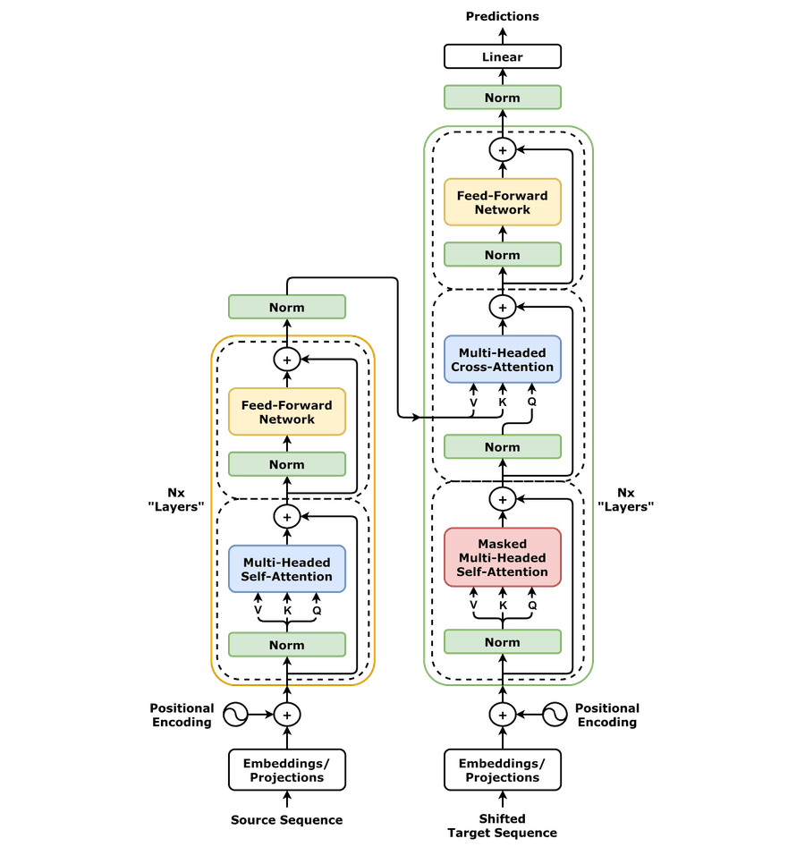
Where the norm goes matters. The original transformer normalised after each addition (post-norm). Most modern models normalise the input of each sub-layer and leave the stream itself untouched (pre-norm, as in Figure 1). Pre-norm keeps a clean path from the top of the model to the bottom, so gradients flow easily and deep stacks train reliably, usually with less careful learning-rate warm-up.
Step 4: Stack them
A model is an embedding layer, then identical blocks (each with its own weights), then a final layer norm and an output layer that turns each token's final vector into scores over the vocabulary. Small models have around a dozen blocks; large ones have many dozens. Here is the canonical full encoder-decoder layout from the literature, drawn in the pre-norm style used today. The decoder-only models behind chat assistants keep just the right-hand column without the cross-attention ( Encoder, decoder and decoder-only models ).

Try it
One pre-norm block in numpy, plus a parameter count for two model shapes:
# A pre-norm transformer block in numpy, then the parameter count of a stack.
import numpy as np

rng = np.random.default_rng(0)
n, d = 4, 16                                   # 4 tokens, width 16

def layer_norm(x, eps=1e-5):
    mu = x.mean(-1, keepdims=True)
    var = x.var(-1, keepdims=True)
    return (x - mu) / np.sqrt(var + eps)       # (learned scale/shift omitted)

def attention(x, Wq, Wk, Wv, Wo):              # single head, causal
    q, k, v = x @ Wq, x @ Wk, x @ Wv
    s = q @ k.T / np.sqrt(d) + np.triu(np.full((n, n), -np.inf), 1)
    w = np.exp(s - s.max(1, keepdims=True))
    return (w / w.sum(1, keepdims=True)) @ v @ Wo

def mlp(x, W1, W2):                            # widen 4x, nonlinearity, narrow
    return np.maximum(0, x @ W1) @ W2

W = lambda *shape: rng.normal(size=shape) * 0.1
Wq, Wk, Wv, Wo = W(d, d), W(d, d), W(d, d), W(d, d)
W1, W2 = W(d, 4 * d), W(4 * d, d)

x = rng.normal(size=(n, d))                    # the residual stream
x1 = x + attention(layer_norm(x), Wq, Wk, Wv, Wo)  # read, add back
x2 = x1 + mlp(layer_norm(x1), W1, W2)              # read, add back
print("stream shape stays", x.shape, "->", x2.shape)
print(f"size of what each sub-layer added: attention "
      f"{np.linalg.norm(x1 - x):.2f}, MLP {np.linalg.norm(x2 - x1):.2f}, "
      f"stream {np.linalg.norm(x):.2f}")

def params(d, layers, vocab, ctx):
    attn, ffn = 4 * d * d, 2 * d * 4 * d       # ignoring biases and norms
    emb = vocab * d + ctx * d
    return attn * layers, ffn * layers, emb

for d_, L in [(768, 12), (4096, 32)]:
    a, f, e = params(d_, L, 50_257, 1024)
    total = a + f + e
    print(f"width {d_:>4}, {L} layers: attention {a / 1e6:7.1f}M  "
          f"MLP {f / 1e6:7.1f}M  embeddings {e / 1e6:5.1f}M  "
          f"total {total / 1e6:7.1f}M  (MLP share {f / total:.0%})")
Output
stream shape stays (4, 16) -> (4, 16)
size of what each sub-layer added: attention 0.79, MLP 1.79, stream 9.74
width  768, 12 layers: attention    28.3M  MLP    56.6M  embeddings  39.4M  total   124.3M  (MLP share 46%)
width 4096, 32 layers: attention  2147.5M  MLP  4295.0M  embeddings 210.0M  total  6652.5M  (MLP share 65%)
Try this:
- Check the shapes: the stream goes in as
(4, 16)and comes out as(4, 16). Every block preserves the shape, which is why blocks can be stacked any number of times. - Compare the sizes in the second line: each sub-layer adds a modest update to a stream that is much larger. Blocks refine the stream rather than replace it.
- Read the parameter counts. Use the formulas below to check one by hand before reading on.
Going deeper
Parameter-count math
Ignoring small biases and norm weights, one block has:
- attention: , each , so ;
- feed-forward: is and is , so ;
- total per block, and for blocks.
Add the token embedding table, vocabulary x , and learned position vectors if the model has them. For width 768, 12 blocks, a 50,257-token vocabulary and 1,024 positions: million in the blocks plus 39.4 million in embeddings, about 124 million. At width 4,096 with 32 blocks the blocks hold about 6.4 billion parameters and the embeddings only 0.2 billion.
Two useful consequences. A forward pass costs roughly 2 floating-point operations per parameter per token (one multiply and one add), which is how training and serving costs are estimated ( Pretraining: next-token prediction , How LLM inference works ). And since the feed-forward layers hold most weights, they are the natural place to add capacity cheaply with a mixture of experts ( Mixture of experts ).
Why residuals matter so much
Without residual connections, a signal would pass through dozens of transformations in sequence, and gradients would shrink or explode on the way back. With them, the gradient has a direct path through the additions to every layer, so a 100-block model is trainable. Residuals also make each block's job easier: it only needs to learn a useful change to the stream, and if it has nothing to add it can learn to add almost nothing.
Reading the stream
Interpretability researchers treat the residual stream as a shared communication channel: early layers write features, later layers read them. Projecting the stream of an intermediate layer through the output layer often already gives sensible next-token guesses, which sharpen as you go up the stack.
Trade-offs
| Option | Wins when | Loses when |
|---|---|---|
| Post-norm (original) | Can reach slightly better results when it trains well | Harder to train deep stacks; needs careful learning-rate warm-up |
| Pre-norm (common today) | Stable training of very deep models; clean residual path | Stream magnitude grows with depth; a final norm is required |
| Wider blocks, fewer layers | More parallel work per layer; fewer sequential steps | Less depth for multi-step composition of features |
| Narrower blocks, more layers | More sequential processing steps | Slower per token at inference; harder to parallelise |
Common mistakes
- Thinking attention holds most of the parameters. In a standard block the feed-forward network has twice as many.
- Forgetting the residual connections when implementing a block from scratch; a deep stack without them barely trains.
- Mixing up where the layer norm goes in pre-norm: it normalises the sub-layer's input, not the stream itself.
- Counting parameters as and forgetting the embedding table, which dominates in small models with large vocabularies.
- Assuming each block does a distinct, human-readable job. Features are spread across many layers.
In the wild
Where you will see this: every modern language model, from small on-device models to frontier models, is a stack of blocks like this one, usually decoder-only, pre-norm, with RMSNorm, a gated feed-forward variant and rotary positions. Vision transformers apply the same block to patches of an image, and speech and protein models reuse it unchanged. When a model card lists "layers", "hidden size" and "heads", it is describing these blocks.
Check yourself
-
What does the residual connection do in a transformer block?
Show answer
B. Adds each sub-layer's output to its input, so information and gradients can pass straight through x <- x + f(LN(x)). The stream keeps everything that was there and gains the sub-layer's update.
-
In one standard block of width d, how many weights do the feed-forward layers have?
Show answer
B. 8d^2 W_1 is d x 4d and W_2 is 4d x d: 4d^2 + 4d^2 = 8d^2, twice the attention's 4d^2.
-
Which sub-layer moves information between token positions?
Show answer
C. Multi-head attention Attention is the only part where tokens read from other tokens. The feed-forward network and norms work on each token separately.
-
A model has width 1,024, 24 blocks and a 32,000-token vocabulary. Roughly how many parameters, ignoring positions, biases and norms?
Show answer
B. About 335 million Blocks: 12 x 1,024^2 x 24 = 302 million. Embeddings: 32,000 x 1,024 = 33 million. Total about 335 million.
Recap
- A block is attention (tokens talk) then a feed-forward network (each token thinks), each with a residual connection and layer norm.
- The residual stream carries each token's vector up the stack; sub-layers read from it and add back.
- Pre-norm normalises each sub-layer's input and keeps a clean residual path, which makes deep stacks stable.
- A block has about 12 d^2 weights, two thirds of them in the feed-forward layers.
- Models are this block stacked dozens of times, plus embeddings at the bottom and an output layer at the top.
Next up
- Build production LLM apps learning path